Introduction to Stable Diffusion Finetuning

I recently had the amazing opportunity to be a speaker at DSC Europe 2023. I was really impressed by how many people asked me to share my slides afterwards, so I decided to summarize my talk in a blog post + add some details.

This post is the first such experience for me. It is more like a gentle overview of the existing methods - their strengths and weaknesses. I hope that it might help someone who is starting their journey into Computer Vision Generative models.

Generative models

Generative models is a special class of models that are able to produce some output signal that has similar characteristics (or a similar distribution) with the data they were trained on. Under the hood, these models estimate the posterior probability of the real data $P(x)$ and they use this knowledge to generate new samples.

Most often, these models are built in a way that allows to incorporate some condition into the generation process, so they estimate $P(x \mid y)$, where $y$ is some conditional signal.

Generative models can be applied to various sorts of target domains - text, audio, images, video, etc. The structure of the target signal influences the model architecture - whether it will operate in autoregressive fashion or not, what layers will be used to build it up, what mechanisms can we to incorporate our conditional signal into the generation process. If we focus on the image generation models, we can come up with the following model taxonomy:

• VAE - Variational Autoencoder. This type of model usually has an encoder-decoder architecture. An encoder significantly compresses the input signal, losing information in the process. A decoder tries to decompress it back to the original input. To make this autoencoder variational, we introduce an even more serious bottleneck into architecture - an encoder outputs some distribution parameters, and the decoder uses these parameters to perform sampling. The most famous representatives are VQ-VAE, VQ-VAE-2, and AutoEncoderKL.
• GAN - Generative Adversarial Network. This type of model consists of two parts - a Generator and a Discriminator / Critic. The Generator produces an output sample, while the Discriminator tries to distinguish the generated sample from the one that came from the real data. The training process looks like a minimax competition between these two models. GANs are prone to various types of problems, but the scientific community has developed various techniques to overcome them. In order to perform the training, these models can use different adversarial losses (minimax loss / NSGAN, LSGAN, EBGAN, BEGAN, WGAN, WGAN-GP). The best known representatives are ProGAN, StyleGAN, StyleGAN2, Alias-Free GAN / StyleGAN3, BigGAN, pix2pixHD, and SPADE.
• NF - Normalizing flow. These models transform a simple probability distribution into a more complex one using a sequence of invertible transformations. They explicitly learn the data distribution $P(x)$, so they can be used for both data generation and density estimation. The most famous representatives are RealNVP, NICE, and Glow.
• Diffusion-based models. These models learn to iteratively denoise a noisy input signal. Their simplicity and ease of training have boosted the generative area in the last 2 years. The best known representatives are ImageGen, DALL-E, DALL-E 2, Kandinsky, and Stable-Diffusion.

In this post, I’ll focus on the diffusion-based models and their fine-tuning.

DDPM

DDPM stands for “Denoising Diffusion Probabilistic models”. They belong to the class of latent variable models, so along with our clean data $x_0$ we assume that there exist latents $x_1, \dots, x_T$ of the same dimensionality as the data.

\[p_{\theta}\left( x_0 \right) := \int p_{\theta} \left( x_{0:T} \right) \mathrm{d} x_{1:T}\]

There are two processes defined for this type of models - one of them is called the forward diffusion process and the second one is called the reverse denoising process.

Denoising Diffusion Probabilistic Models, arXiv:2006.11239

Forward diffusion process

The diffusion process consists of several steps, at each step some random Gaussian noise is added to the input signal, resulting in a gradual degradation of the signal to pure noise.

\[q\left ( x_{1:T} \right ) := \prod_{t=1}^{T} q \left ( x_{t} \mid x_{t-1} \right )\]

\[q \left ( x_{t} \mid x_{t-1} \right ) := \mathcal{N} \left ( x_{t} ; \sqrt{1 - \beta_t} x_{t-1}, \beta_t \mathcal{I} \right )\]

where $\beta_1, \dots, \beta_T$ is a variance schedule for the Gaussian noise.

One of the cool features of the forward process is the fact that we can sample $x_t$ at any time $t$ in a single step:

\[\alpha_t := 1 - \beta_t\]

\[\bar{\alpha}_t := \prod_{s=1}^{t} \alpha_{s}\]

\[q \left( x_t \mid x_0 \right) = \mathcal{N} \left( x_t; \sqrt{\bar{\alpha}_t} x_0, (1 - \bar{\alpha}_t) \mathcal{I} \right)\]

Reverse denoising process

The second process is the part where the magic happens. This process is parameterized by some neural networks $\mu_{\theta} \left( x_t, t \right)$ and $\Sigma_{\theta} \left( x_t, t \right)$ whose predictions we use to gradually remove noise from the input signal until all the noise is removed. So, basically, this process acts as a parameterized Markov chain.

\[p_{\theta} \left( x_{0:T} \right) = p \left( x_T \right) \prod_{t=1}^{T} p_{\theta} \left( x_{t-1} \mid x_{t} \right)\]

\[p_{\theta} \left( x_{t-1} \mid {x_t} \right) = \mathcal{N} \left( x_{t-1} ; \mu_{\theta} \left( x_t, t \right), \Sigma_{\theta} \left( x_t, t \right) \right)\]

Usually, for most of the models, $\Sigma_{\theta} \left( x_t, t \right)$ is not trained at all and is just fixed to $\Sigma_{\theta} \left( x_t, t \right) = \beta_t \mathcal{I}$.

Stable Diffusion

High-Resolution Image Synthesis with Latent Diffusion Models, arXiv:2112.10752

Stable Diffusion is a text-conditioned image generation model, which was produced by Runway ML and Stability AI, with the help of CompViz group from LMU Munich.

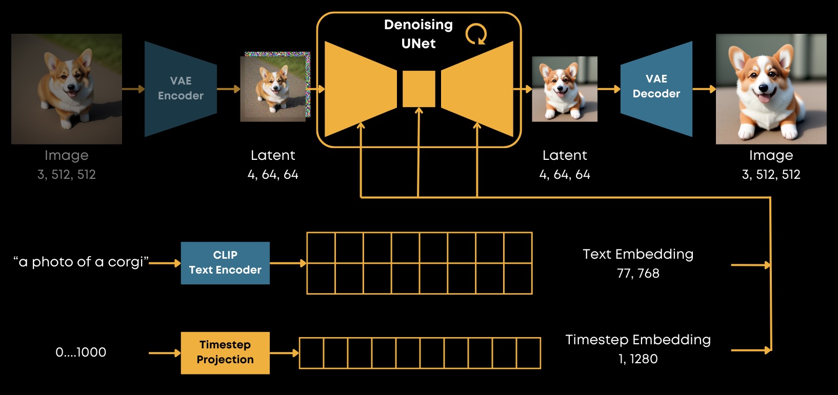
This model belongs to the class of so-called latent diffusion models. In order to minimize the computational cost for both training and inference, it incorporates a pre-trained Variational Auto-Encoder model that is able to significantly compress images to an entity called “latent”. You can think of it a minimized version of an image. So, instead of operating in an image pixel space, this model operates in latent space.

It also utilizes some other pre-trained models like OpenAI CLIP for encoding the provided text conditioning.

The most important part of the model is, of course, is the denoising UNet. It consists of several downsample blocks, followed by the mid block, and several upsample blocks. Each of these is a mixture of resnets and cross-attention blocks. The latter blocks are used to condition the model with some external signal, such as text embeddings.

Thus, this model accepts some noisy latent as input, as well as some text embedding and the current timestep at which is operating, and can produce one of the following results:

1. $\epsilon$-prediction. The prediction is just an estimate of the noise in the image.
2. $x_0$-prediction. The prediction is the estimate of the final $x_0$ at the current step.
3. $v$-prediction. The prediction of the model is $v := \alpha_t \epsilon - \sigma_t x$. This representation allows to significantly reduce the number of sampling steps and has been used in this paper as a method to model distillation.

You can take a look at the original code for loss calculation here:

def get_v(self, x, noise, t):
    return (
        extract_into_tensor(self.sqrt_alphas_cumprod, t, x.shape) * noise -
        extract_into_tensor(self.sqrt_one_minus_alphas_cumprod, t, x.shape) * x
    )

def p_losses(self, x_start, t, noise=None):
    noise = default(noise, lambda: torch.randn_like(x_start))
    x_noisy = self.q_sample(x_start=x_start, t=t, noise=noise)
    model_out = self.model(x_noisy, t)

    loss_dict = {}
    if self.parameterization == "eps":
        target = noise
    elif self.parameterization == "x0":
        target = x_start
    elif self.parameterization == "v":
        target = self.get_v(x_start, noise, t)
    else:
        raise NotImplementedError(f"Parameterization {self.parameterization} not yet supported")

    loss = self.get_loss(model_out, target, mean=False).mean(dim=[1, 2, 3])

The denoising Unet is also a time-aware model - it accepts a time step projected into some vector, either through Positional Encoding or Fourier Encoding. It can be simply added to hidden states inside ResNet blocks, through scale-shift renormalization, through AdaGroupNorm, or through SpatialNorm. Stable Diffusion uses simple addition of timestep embedding to hidden states inside ResNet blocks.

Stable Diffusion versions

It is worth mentioning that Stable Diffusion has been developed iteratively. Currently there are 4 major versions:

1. Stable Diffusion v1.1 - v1.5 (CompViz repo, RunwayML repo). The training was performed on a subset of LAION-Aesthetics V2 in 512x512 resolution and the model uses $\epsilon$-prediction approach.

2. Stable Diffusion v2.0 - v2.1 (StabilityAI repo). The training was performed on a subset of LAION-5B in 768x768 resolution and the model uses $v$-prediction approach. Also, the authors retrained the model from scratch and used larger version of OpenCLIP instead of OpenAI CLIP.

3. Stable Diffusion XL (StabilityAI repo, arXiv:2307.01952). The model has a slightly different architecture - two stage generation (base + refiner), additional training and inference tricks (like SDEdit). The training was performed in 1024x1024 resolution and the model uses $\epsilon$-prediction approach.

4. Stable Diffusion 3 (blogpost, arXiv:2403.03206). This model is not open-sourced yet, but it is available through an API and it shows incredible results. The main differences lie in the changed model architecture (it uses DiT instead of Unet and uses 3 different text encoders, during training and inference the text condition is processed in parallel with latents, the training is based on Rectified Flow).

Despite the fact that the base Stable Diffusion v1.5 base model is now relatively old, it is still quite actively used by the community. There are tons of different checkpoints compatible with v1.5, you can take a look at the filtered model list on CivitAI.

Stable Diffusion implementations

There are 2 widely used implementations of the Stable Diffusion models:

1. LDM implementation. This is the original implementation made by the CompViz/RunwayML/StabilityAI. A lot of projects and research papers are based on or use this implementation (e.g. k-diffusion).

2. diffusers implementation. This is a reimplementation of the original code, which is compatible with all the HuggingFace ecosystem (you can automatically load the models from the hub, get single line of code serialization and de-serialization, but to use LDM-based checkpoints you may need to use diffusers conversion scripts).

In my personal opinion I would say that diffusers implementation is more production ready, however sometimes you may be missing the latest and greatest methods developed, but it is a great opportunity to add them by yourself (they have a great contribution guide).

Stable Diffusion ecosystem

The community has developed lots of instruments that help one to interact with Stable Diffusion. Some of them are paid ones, and some of them are completely open source:

1. AUTOMATIC1111 / Stable Diffusion web UI - >100K starts on GitHub. It allows you to interact with Stable Diffusion through a simple but effective browser UI. At first glance, it may seem a bit simplified, but it is very powerful, and you can also extend it with an impressive list of extensions.

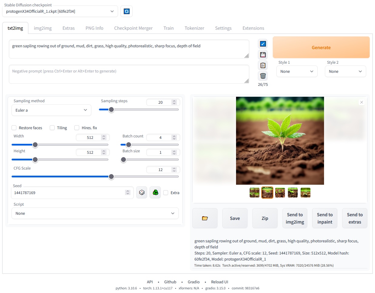
   Stable Diffusion web UI

2. ComfyUI - >20K stars on GitHub. This interface is more advanced - it gives you the ability to build data processing as an acyclic directed graph. It is more flexible compared to webUI, but you need a deeper understanding of image generation pipelines and other models.

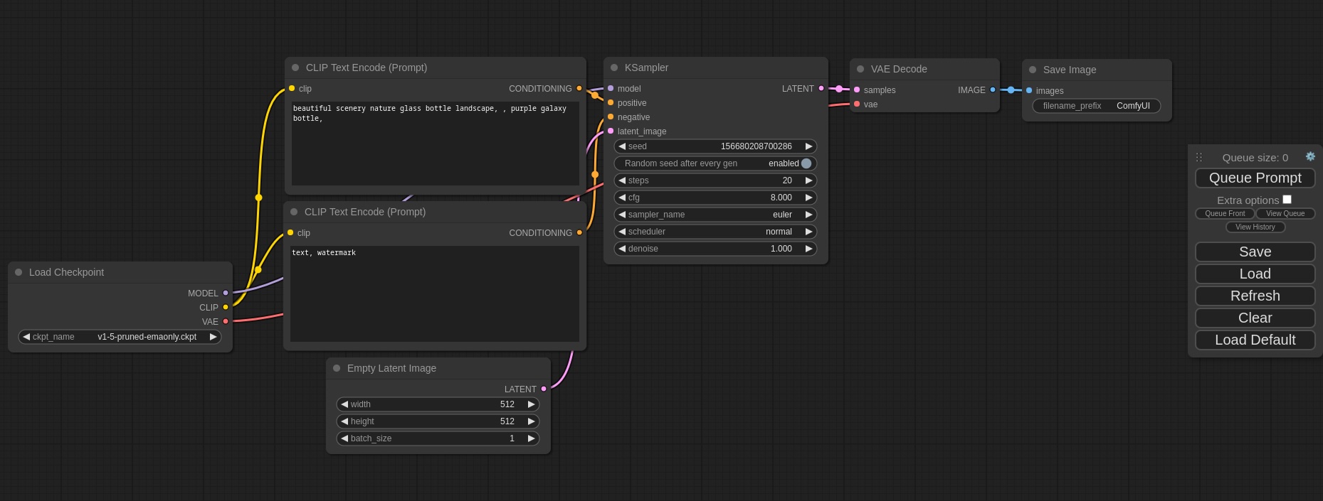
   ComfyUI

Fine-tuning image Generation model

So, what does it mean to fine-tune an image generation model?

Image Generation model fine-tuning

Usually, this means that we want to refine some existing generations to improve the quality or incorporate some new object into a generation that the model has not seen during training.

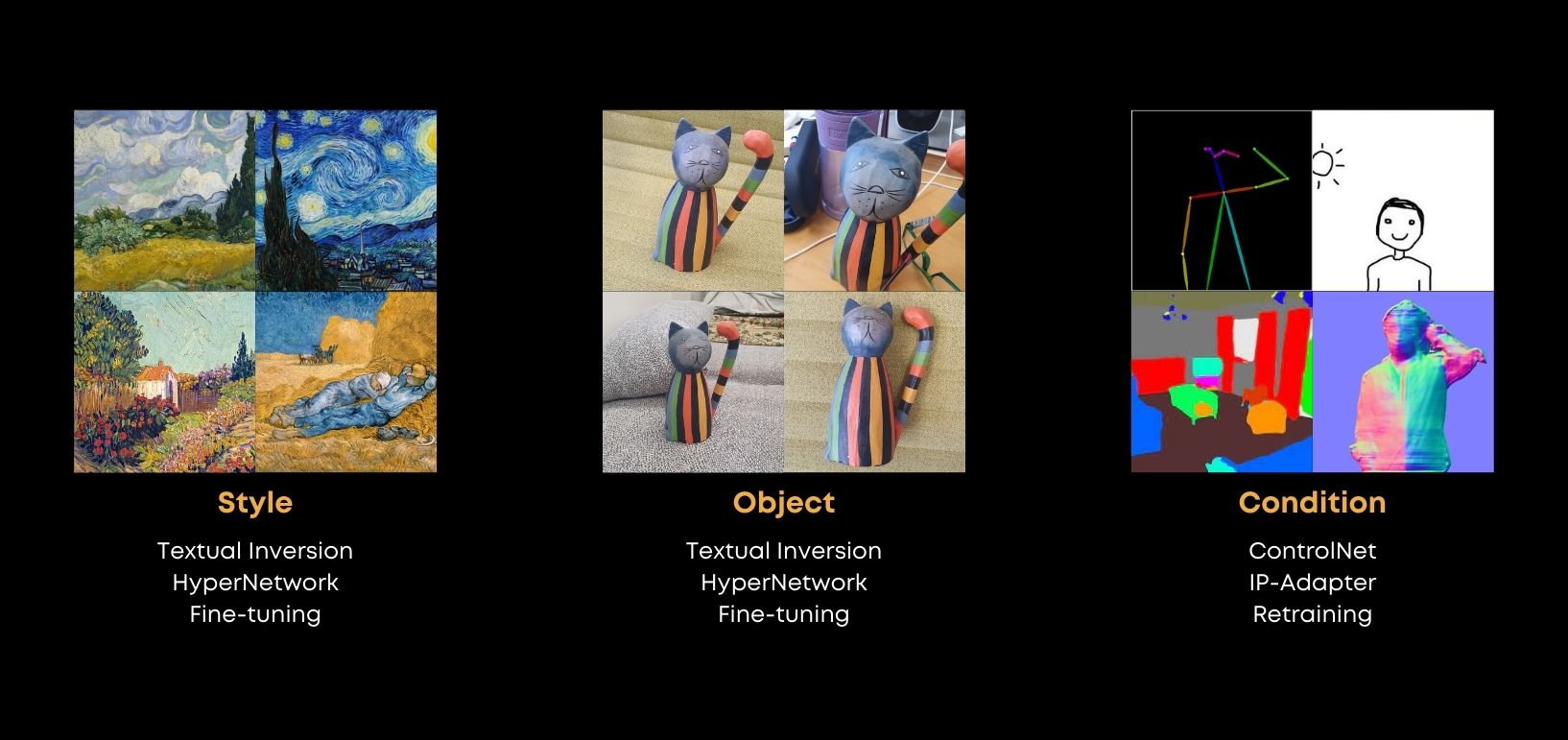
There are several approaches to do this, such as Textual Inversion, HyperNetworks, or Full or partial fine-tuning that will be covered in this article.

But sometimes we may even want to incorporate some new conditional type of information into the existing model checkpoint. So, there are several solutions like ControlNet’s, IP-Adapter’s that do not require full model retraining.

In this article, I’ll focus on methods that allow you to incorporate style or object into the image generation pipelines.

Textual Inversion / Textual Embedding

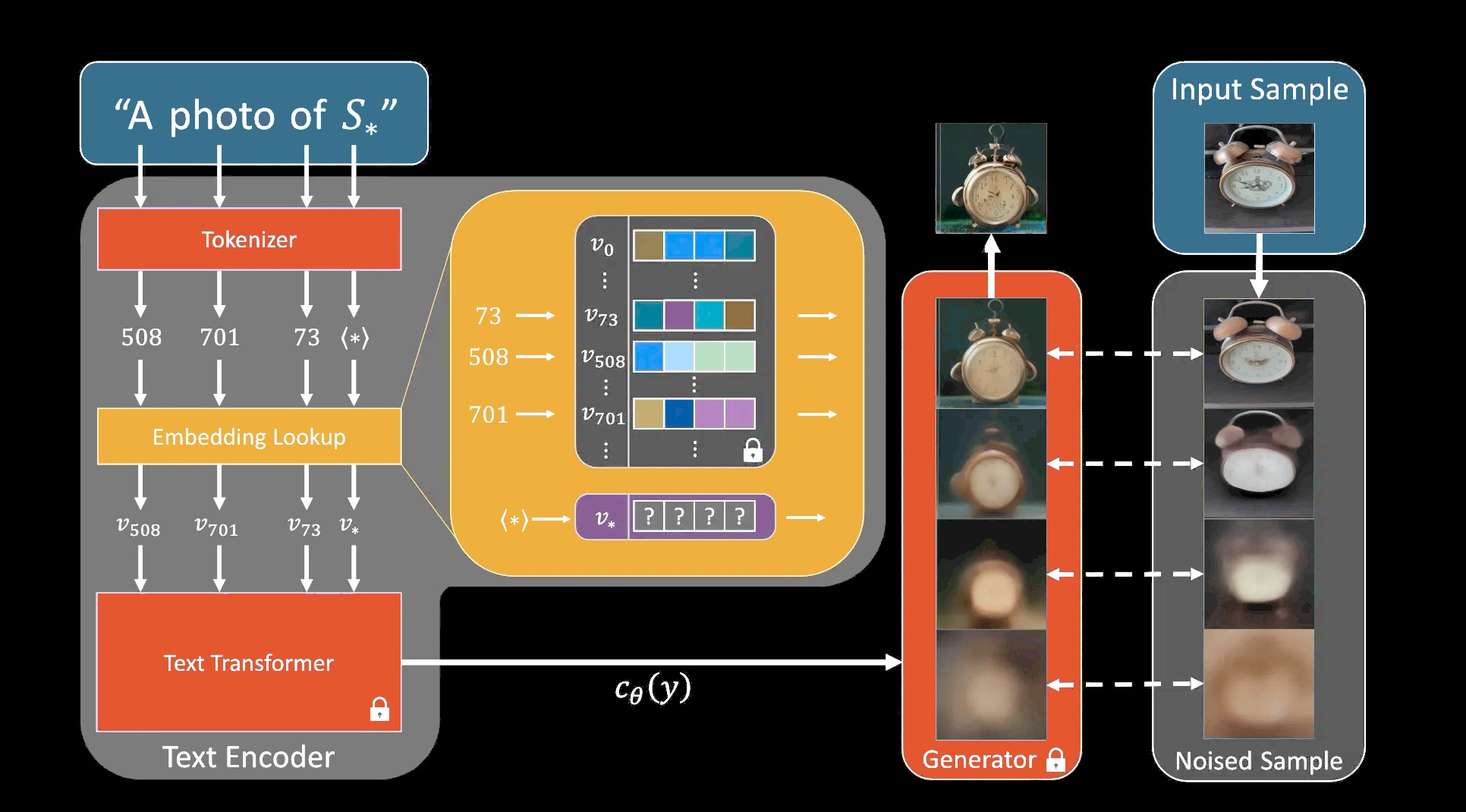
An Image is Worth One Word: Personalizing Text-to-Image Generation using Textual Inversion, arXiv:2208.01618

Since we are working with a text-conditioned image generation model, we can make a simple assumption that a precise object or style text description might help us during generation.

So, we can add some new tokens to the text model and just fine-tune them, leaving the rest of the model fixed. You can think of this process as finding the best single word or set of words that accurately describes your object or style.

The fine-tuning process works as follows:

1. You add new embeddings to the text model and initialize them with an initial value - it can be something close to the concept you are training.
2. You take an input sample of your concept and you add some noise to it according to the noise schedule.
3. Then you pass this noisy sample and your text description into the generator, it outputs the predicted noise, then you compare it to the added noise with mean squared error, and you backpropagate the gradients back to the new embeddings you added.

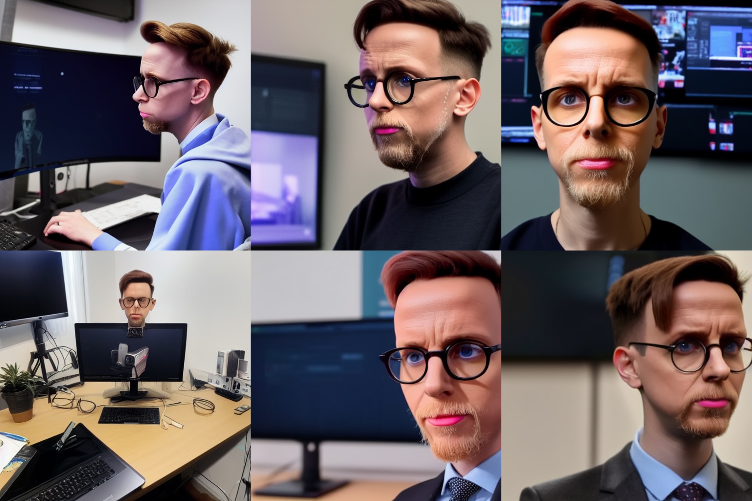
Here are the results of textual embedding trained on my own personal photos:

Textual Inversion trained on my personal photos

You can see that the output results are not very stable, they don’t look like a real person’s photo. From my experience, I see several points of improvement here:

1. You should use a good starting initialization for newly added embeddings. For example, if you are trying to train an embedding that represents a specific person, use the name of a famous person that looks similar. In this case, you can even reduce the learning rate, train faster and get more consistent results. However, be aware that some textual inversion training scripts (like diffusers textual_inversion.py) may not allow you to provide multiple tokens for initialization.
2. Sometimes, when using a higher learning rate, even a good starting initialization may not help. You can see that current embeddings can provide messy results, or even generate objects that are not related to your training data. In my opinion, this is related to the effect of diffusion loss gradients for unconstrained learnable embeddings. I have done several successful experiments, that show that adding some kind of regularization for learnable embeddings that helps them stay in the distribution of other embeddings may greatly help overcome this problem (I used MSE between the mean norm of the learnable embeddings and the mean norm of all other clip encoder embeddings).

Pros:

• Very lightweight. You only need to train a single layer of a model. Then you can store only the embeddings you’ve trained (their weight can range from a few kilobytes to several hundred of kilobytes).
• Plug and play with different checkpoints. If multiple checkpoints use the same text encoder but different UNets - the produced embeddings could be easily reused between them.

Cons:

• More of a refinement method. This approach doesn’t allow us to incorporate concepts that differ a lot from the training data.

HyperNetwork

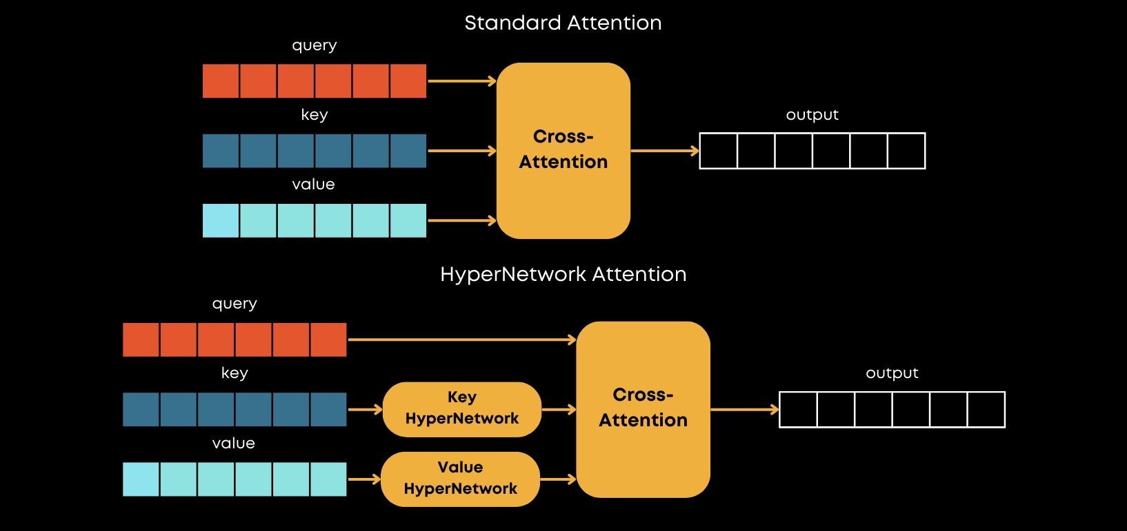
NovelAI Improvements on Stable Diffusion, Blog

Regarding the HyperNetwork approach - you may be familiar with the approach with the same name that Google introduced in 2016.

Google’s main idea was to build a neural network that predicts the weights for another network.

So, in terms of HyperNetworks for Stable Diffusion, the approach is quite different. It was presented by NovelAI in one of their blogs and the main idea is to modify keys and values in Cross-Attention layers with some MLPs that are called HyperNetworks.

The training process is the same as for Textual Inversion (image noising, passing data through UNet).

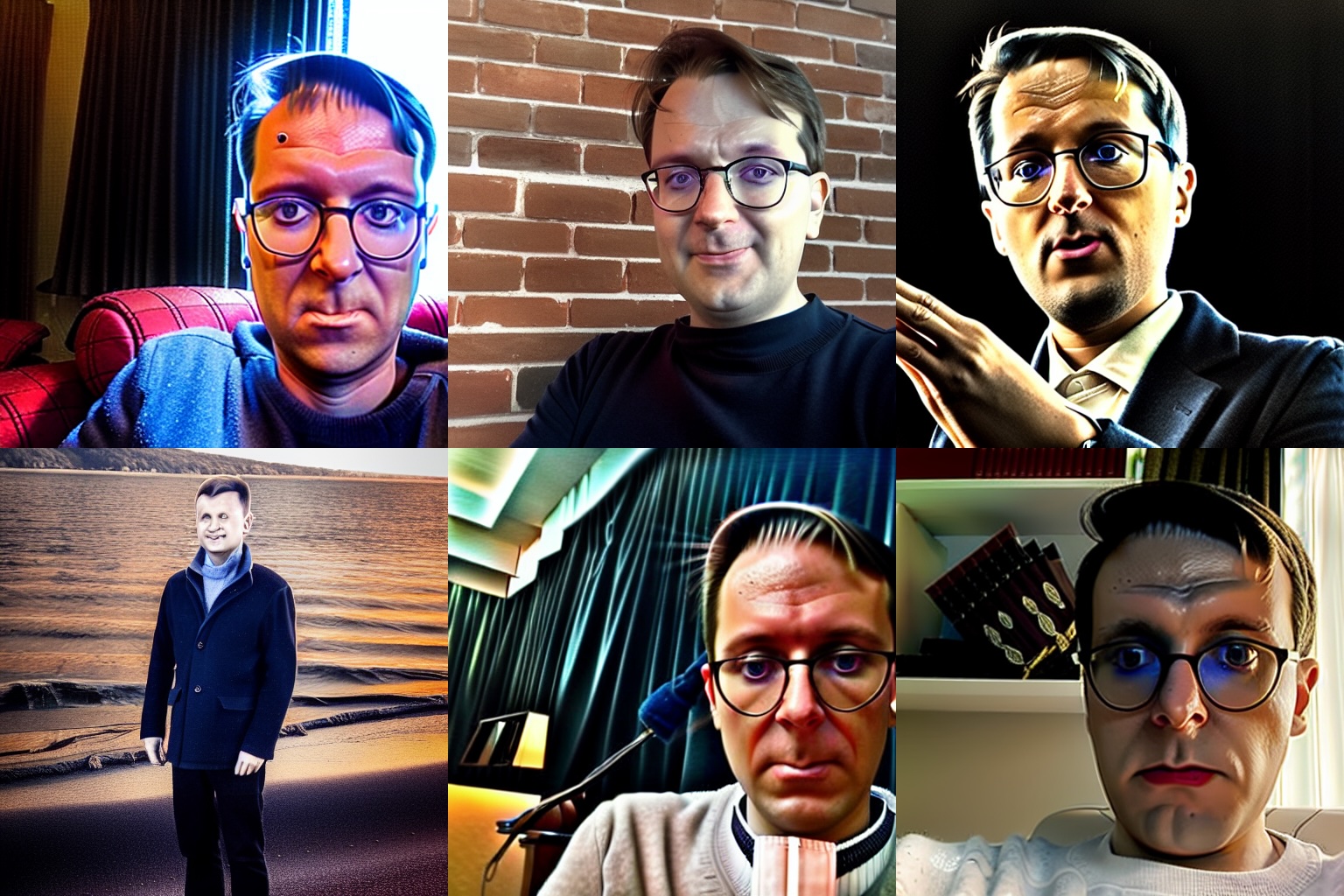
Here are the outputs of HyperNetwork trained on my own personal photos:

HyperNetwork trained on my personal photos

Pros:

• Similar to fine-tuning. This approach modifies all cross-attention layers. So, from this perspective, it is more similar to full model fine-tuning compared to the Textual Inversion.

Cons:

• Poor convergence. Based on empirical studies, it is hard to train hypernetworks.
• Only modifies cross-attention layers. Other important layers like Linear, Conv2d are not modified in any way.
• Checkpoint-dependent approach. A HyperNetwork trained on one checkpoint cannot be transferred to another checkpoint due to differences in cross-attention activations.

Despite the fact that HyperNetworks produce unsatisfactory results, I still think that this approach could have gotten more attention, if the implementation of this method had been open-sourced rather than re-implemented by a leaked code (reddit post, webui issue). In my opinion, the HyperNetwork approach for Stable Diffusion seems quite similar to the later introduced IP-Adapter, which shows very promising results.

Dreambooth

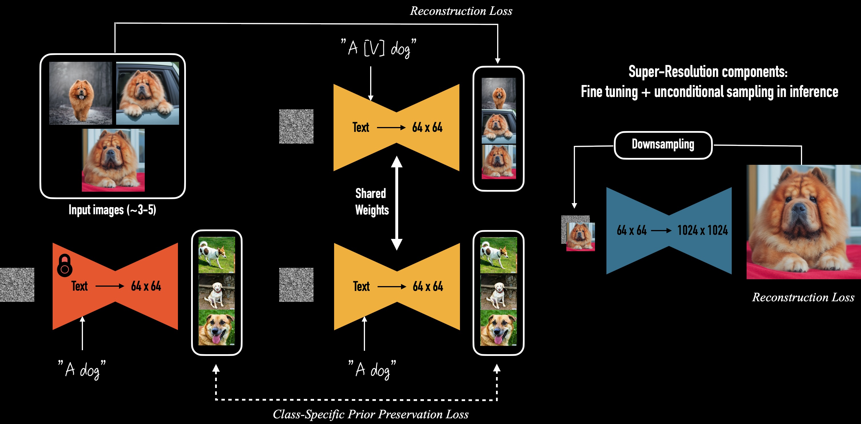
DreamBooth: Fine Tuning Text-to-Image Diffusion Models for Subject-Driven Generation, arXiv:2208.12242

Regarding the fine-tuning approach, everything may seem straightforward - you just fine-tune your model on some images, you pass in some text descriptions, and that’s it, but in reality, diffusion models are prone to so-called “catastrophic forgetting”.

It’s a situation where the model is able to produce your style or object, but it forgets everything it was trained on. To deal with this, Google came up with a simple idea - they add some regularization images to the training set along with the target fine-tuning dataset. This is called the Dreambooth approach, and it is de-facto the standard approach to model fine-tuning nowadays.

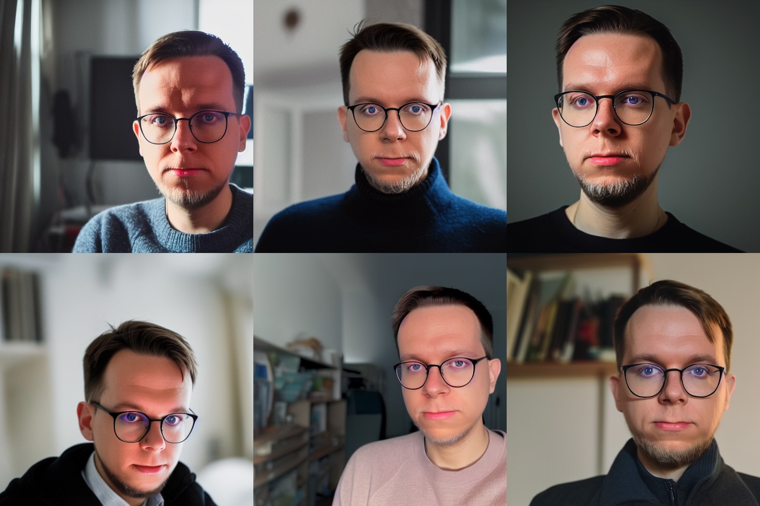
Here are the outputs of Dreambooth trained on my own personal photos:

Dreambooth trained on my personal photos

Pros:

• Produces the best results. Dreambooth produces the best results compared to other methods (Textual Inversion, HyperNetwork).

Cons:

• Heavy approach. It is quite heavy in terms of GPU memory usage, of course, you can fine-tune only some layers of the model and fix the others, but it is quite hard to tell which layers affect performance the most.
• Large checkpoint size. After training you get a checkpoint with the same size as the full model, so if you want to experiment with other base checkpoints, you may have to retrain everything from scratch.

As you can see, that the Dreambooth approach produces the best results over all other methods, but this approach is quite heavy - you need to optimize all model layers, so it may be difficult to perform this training on consumer hardware.

Finetuning

Let’s spend some time analyzing the amount of memory required for Stable Diffusion fine-tuning.

By 2024 standards, basic Stable Diffusion is a relatively small model with just over 1 billion parameters in total:

• VAE - 84M parameters
• UNet - 860M parameters
• Text Encoder - 123M parameters
• Total - 1.0B parameters

It’s also worth noting that the variational autoencoder part is almost never trained at all, but you may notice that it’s the smallest part of this ensemble.

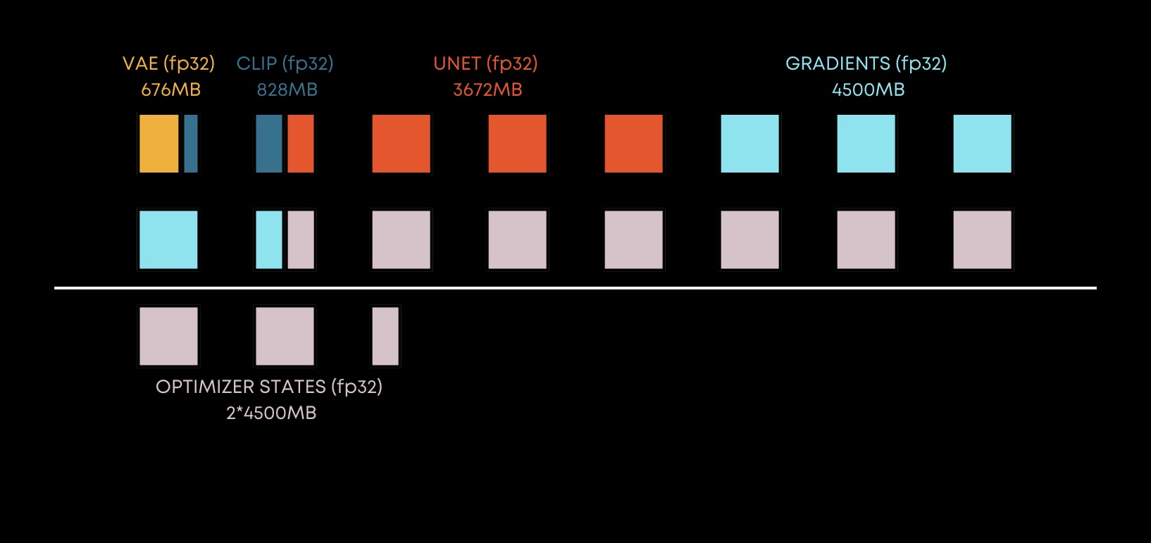
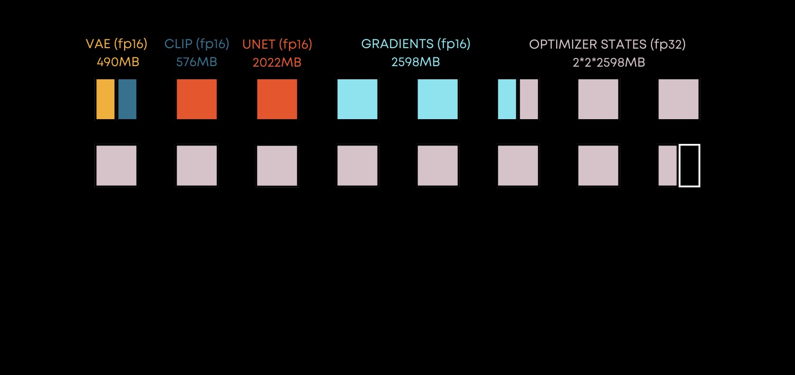
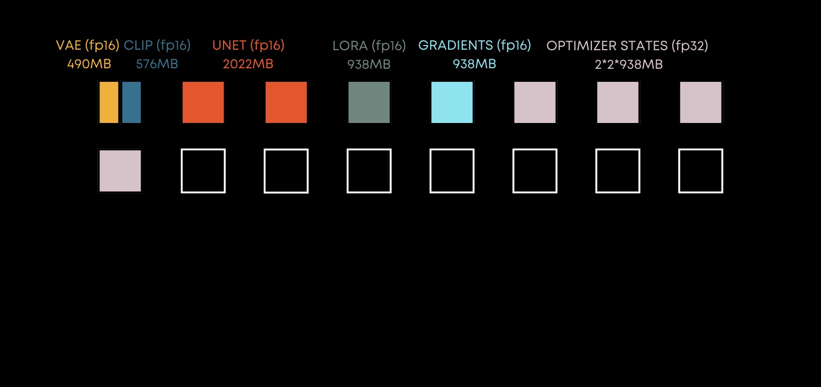
Let’s take a look at the memory consumption during model fine-tuning on some consumer hardware. Suppose that we have a GPU with 16GB of VRAM. To visualize the memory consumption, I decided to create a visualization inspired by a fantastic Predibase tutorial on Efficient Fine-Tuning for Llama-v2-7b on a Single GPU. Each square in the images below represents 1GB of VRAM.

A small disclaimer: my calculations may not be very precise and accurate, they do not take into account additional memory consumption by torch, memory allocation strategies, caching, intermediate activations, etc., but the overall picture should be fine.

Fine-tuning / Dreambooth - Memory footprint - FP32

Overall, in fp32 all the models parameters take around 5GB of VRAM. In order to perform optimization, you need to store the gradients somewhere, so basically you need the same amount of memory as the trainable parameters take (we don’t fine-tune VAE), so in case of Stable Diffusion it’s something around 4.5GB of VRAM.

And last but not the least part is the optimizer. So, if you use the Adam, which is the most common optimizer right now, it has pretty heavy memory consumption. It almost consumes memory equal to 2x the number of trainable parameters, so in this case, it is around 9GB of VRAM.

This is the moment when we are already out of memory on our GPU. We need to do something about it to train the model, so the first obvious thing to do is to switch from fp32 to fp16 precision.

Fine-tuning / Dreambooth - Memory footprint - FP16

When we switch to fp16 precision, out memory consumption for models and gradients decreases almost by half, but I am pretty sure that we still need to store optimizer states in fp32.

At this point, we’re able to store almost everything on the card, but we haven’t taken into account the intermediate activations in the model, so we may not be able to train with a batch more that 1 with using gradient accumulation or other techniques.

So, are there any other methods that would allow us to fine-tune the model and reduce memory consumption?

Parameter-Efficient fine-tuning

Scaling Down to Scale Up: A Guide to Parameter-Efficient Fine-Tuning, arXiv:2303.15647

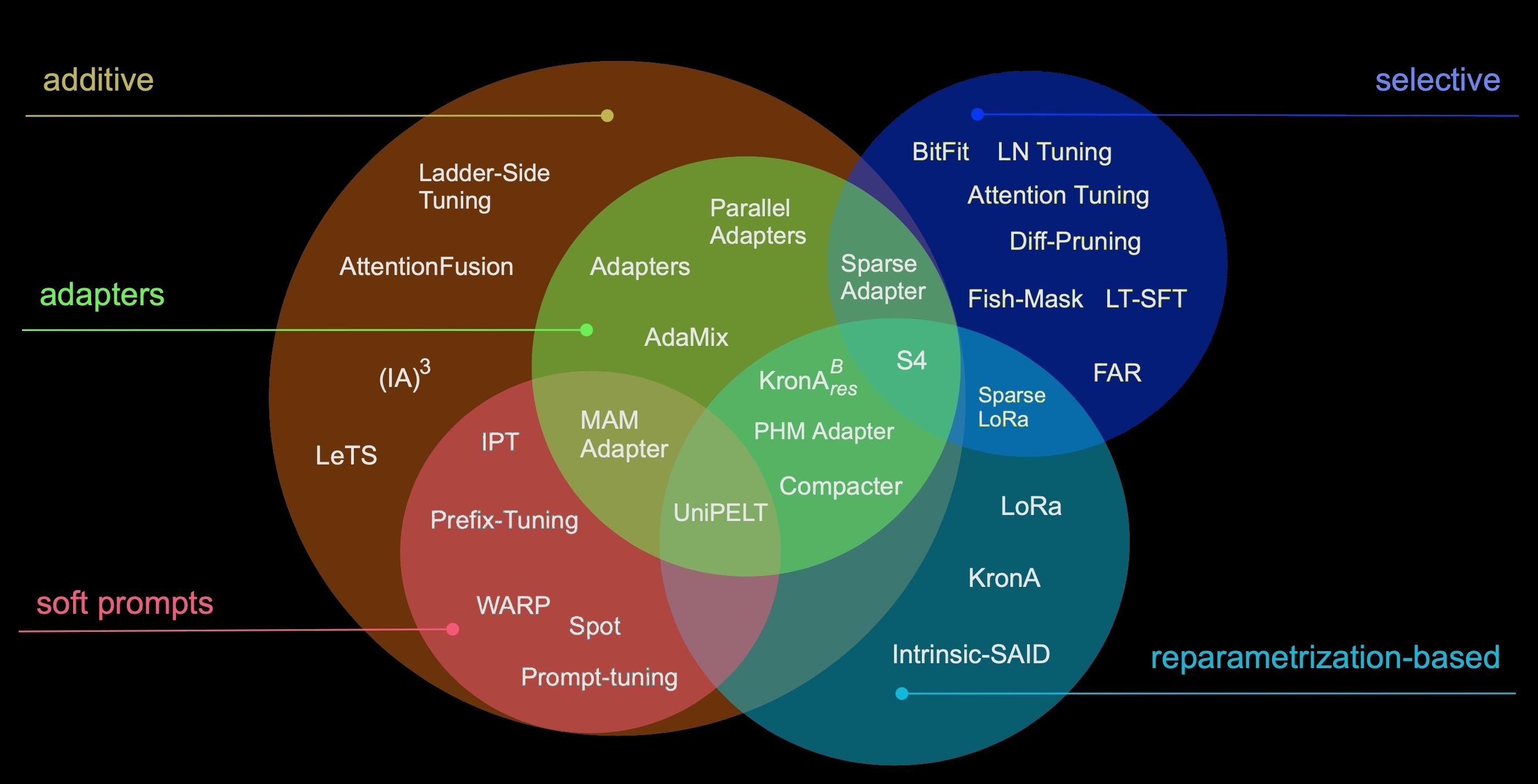
Today there exist various methods that allow you to fine-tune only a small number of parameters and get similar performance compared to full model fine-tuning. These methods may range from very lightweight, cheap, and efficient methods down to heavy and precision-oriented methods.

The most popular method, and the one that has been most widely adopted by the Stable Diffusion community, is the LoRA method, so we’ll focus on that.

LoRA

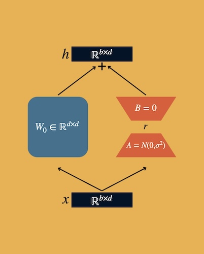
LoRA stands for Low-Rank-Adaptation and the beauty of this approach lies in its simplicity.

LoRA architecture

$h = W_0x + \Delta Wx = W_0x + BAx$

We introduce some additional matrices $B$ and $A$ alongside the base weights matrix $W$. These matrices are smaller than the base weight matrix $W$, but their dot product is the same size as the base weight matrix (e.g. $W \in \mathbb{R}^{N \times M}$, $B \in \mathbb{R}^{N \times r}$, $A \in \mathbb{R}^{r \times M}$, $r$ is the rank hyperparameter, so the more $r$ is - the bigger the LoRA gets).

This approach is pretty cool, it allows us to train different adapters for various types of models. It also reduces memory consumption, and there are a lot of empirical studies that show that models trained with LoRAs get almost the same accuracy as fully fine-tuned models.

1. A pre-trained model can be shared and used to build many small LoRAs.
2. LoRA makes training more efficient in terms of VRAM and provides quality comparable to full fine-tuning.
3. LoRA matrices can be merged with the base weights when deployed, so it won’t influence the inference latency at all.
4. LoRA can be extracted from two base model checkpoints. You just need to calculate $\Delta W$ and decompose it with something like SVD (Singular Value Decomposition). This approach can also be used to decrease the rank of a trained LoRA with the loss of precision.
5. LoRA can be applied to different layers - Embedding, Linear, Convolutional, 1d, 2d, 3d, etc. So it can be attached to various sorts of models (Classification, Computer Vision, Text Generation, etc.).

LoRA - Memory footprint

LoRA Memory Footprint

In terms of memory footprint, LoRA greatly reduces the number of trainable parameters, resulting in less memory for gradients, less memory for optimizer states, and more memory to store activations, to increase effective batch size; in our toy example we have more than 6 gigabytes free from our 16 gigabytes card.

We can also see, that the LoRA output size for Stable Diffusion is significantly smaller compared to the full Stable Diffusion checkpoint. Of course, the LoRA size depends on the rank, but in general it ranges from several megabytes to several hundred megabytes:

• 11MiB - rank 8
• 21MiB - rank 16
• 41MiB - rank 32
• 82MiB - rank 64
• 163MiB - rank 128

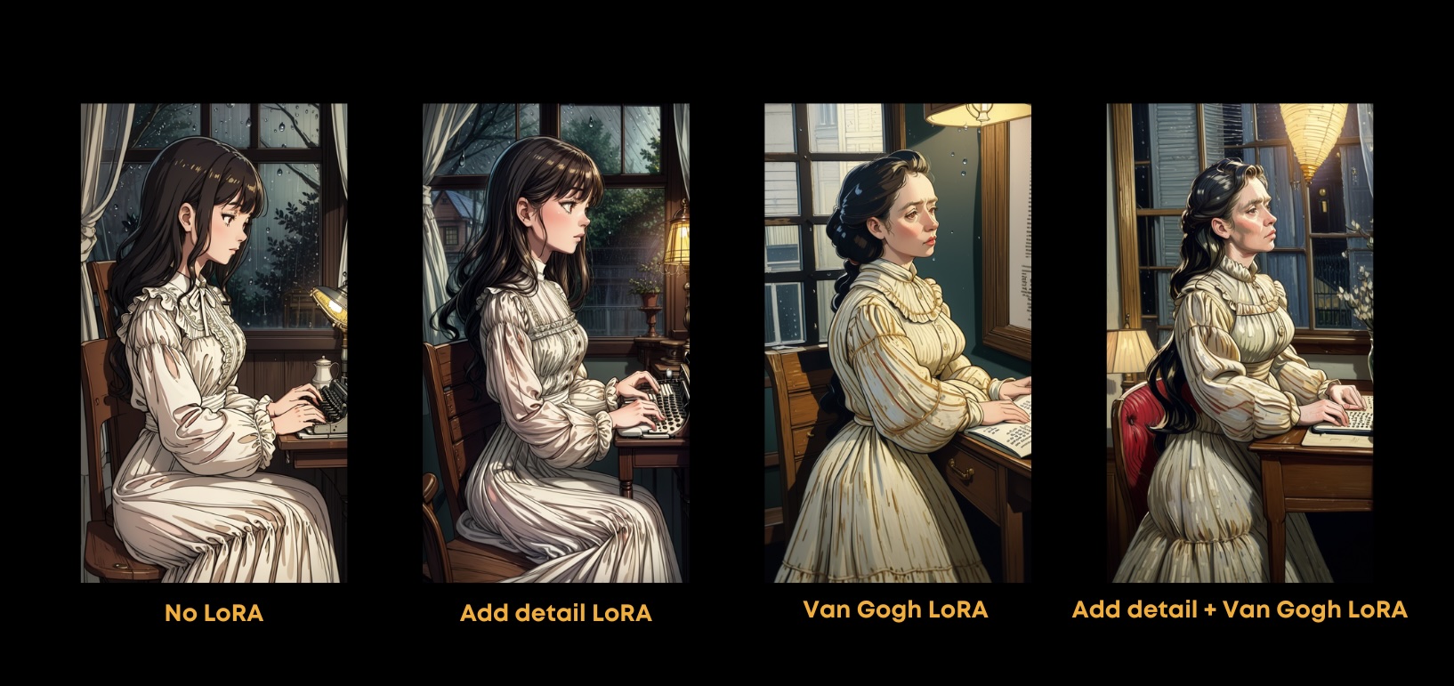
Mixing LoRAs

Mixing LoRAs

Also, in terms of Stable Diffusion, you also get the ability to mix different LoRAs (or other adapters) together to get a unique style, like in this example where I tried to mix a detail tweaker Lora with Van Gogh style Lora.

LoRA - Implementations

Aside from the original Microsoft LoRA implementation for LLMs, there are other popular implementations (some of which are not limited to Stable Diffusion)

• kohya-ss - IMHO, this is the most advanced implementation of LoRA, made specifically for Stable Diffusion and Stable Diffusion XL. It includes a lot of helper code around training data preprocessing, well-working heuristics, multi-resolution training, etc. This implementation can also use other adapters such as LyCORIS (LoHa/LoKr).
• HuggingFace diffusers - this is an official implementation for HuggingFace diffusion models. Although the current implementation may lack some of latest and greatest features here, it is quite solid and well integrated with this framework.
• HuggingFace peft - this is an implementation from HuggingFace that can be used with various types of models (not limited to Stable Diffusion and image generation at all) - they have good tutorials for using the adapters for image classification and segmentation, token classification, automatic speech recognition, etc. It is also well integrated with transformers and diffusers frameworks and has a lot of other adapters implementations.

LyCORIS - alternative implementations for low-rank-adaptation

Navigating Text-To-Image Customization: From LyCORIS Fine-Tuning to Model Evaluation, arXiv:2309.14859

I would also like to mention that the community has come up with different types of adapters except LoRA.

There exists a library for fine-tuning called LyCORIS which has some alternative implementations for different adapters - LoHa and LoKr.

The main difference between these adapters and the plain LoRA lies in the matrix decomposition, which is used during training and inference (they use Hadamard and Kronecker products, respectively). It is noted, that classical low-rank decompositions suffer from limited representational power, so these two matrix products may theoretically help to achieve even better quality with fewer trainable parameters compared to basic LoRA methods (which only use simple matrix multiplication).

LoHa (Low-rank Hadamard product Adaptation) is based on the ideas of the FedPara paper. One of the advantages of LoHa is that the maximum rank of the resulting matrix is larger than the one in LoRA.

LoKr (Low-rank Kronecker product Adaptation) is similar to KronA paper. One of the advantages of LoKr is that when using the Kronecker product, its multiplicative nature results in the multiplication of the ranks of the decomposition matrices.

For both this adapters LyCORIS provides a special type of Conv2d decomposition which helps to reduce the number of trainable parameters for convolution layers.

Conclusions

In conclusion, I would like to mention that the field of image generation is developing very rapidly, new approaches are published every day, and some existing approaches become obsolete very quickly.

Nevertheless, such approaches as Textual Inversion / Dreambooth / LoRA are still key components in more advanced and more complex ones. In my opinion, LoRA methods provide a good compromise between accuracy and hardware requirements and allow us to solve a wide range of tasks by reducing the required computing power, and you should definitely try to use them in your daily tasks.

Feel free to share your thoughts (or the topics in image generation that you would like to learn more about) in the comments section below!